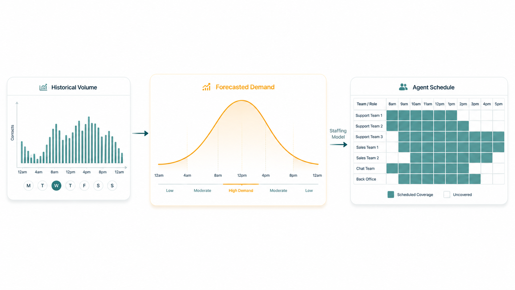
Call center forecasting predicts contact volume at a granular interval level — typically 15 or 30 minutes — using historical patterns, trend analysis, and known events. Scheduling converts that forecast into a staffing plan by calculating how many agents are needed in each interval to meet a defined service level target. Together, they are the core operational disciplines of contact center workforce management.
This article focuses on forecasting and scheduling in depth. For the broader workforce management context — including intraday management, adherence tracking, and WFM as an organizational practice — see What Is Call Center Workforce Management?.
Getting forecasting and scheduling right is the central operational challenge of running a contact center at scale. Overstaff and labor cost climbs. Understaff and wait times rise, abandonment increases, service levels fall, and agents experience unsustainable workloads. The goal is matching supply (available agents) to demand (contact volume) as closely as possible across every interval in the operating day.
Contact volume forecasting
What you are predicting
A contact center forecast does not predict total daily volume as a single number — that is not granular enough to be useful for scheduling. The working unit is the interval: 15 minutes or 30 minutes. A forecast tells you: on Thursday at 10:30 AM, we expect approximately X contacts to arrive. A schedule built on that forecast needs to have enough agents available at 10:30 AM, specifically, to handle X contacts at the service level target.
This interval-level demand prediction is what separates contact center workforce management from general headcount planning. You could know your weekly volume within a few percent and still be significantly overstaffed at 9 PM on Tuesday while being severely understaffed at 11 AM on Monday.
Historical data as the foundation
Most volume forecasting starts with historical contact data. If you handled a certain number of calls on Monday mornings over the past several months, that pattern — adjusted for trend and seasonality — is the starting point for predicting next Monday morning's volume.
The historical data you need includes:
- Volume by interval: Total contacts received in each 15 or 30-minute period, for each day of the week, over a period long enough to reveal weekly and seasonal patterns
- Volume by channel: If you handle calls, chats, emails, and callbacks, each channel has its own volume pattern and may require separate forecasts
- Volume by queue or contact type: If different types of contacts route to different teams or require different handle times, splitting the forecast by type produces more actionable scheduling outputs
Trend analysis and seasonality
Raw historical volume is usually not a perfect template for future volume. Two adjustments are commonly needed.
Trend: Contact centers generally see some growth or decline in volume over time. If your weekly volume grew over the past year, simply applying last year's pattern without adjusting for the underlying trend will produce a forecast that is systematically low.
Seasonality: Most contact centers have predictable seasonal patterns. Retail support spikes around holidays. Healthcare enrollment centers are busiest during open enrollment periods. Financial services see higher volume at end of month and at tax time. A forecast that does not account for known seasonal patterns will repeatedly underestimate volume at predictable times of year.
Known events and external factors
Historical patterns cannot account for future events that have no historical precedent. A product launch, a price change announcement, a marketing campaign, a service outage, or a billing cycle issue can drive contact volume well above forecast levels. Effective forecasting programs maintain a planning calendar that captures known upcoming events and adjusts volume estimates accordingly.
External factors — weather events, news cycles, regulatory changes — may also affect volume in ways that are hard to predict systematically. The forecasting process needs a mechanism for human judgment to override the model when there is good reason to expect unusual volume.
EaseDial Analytics
Historical call volume, interval-level reporting, and queue performance data — the foundation for better forecasting decisions.
From forecast to staffing requirements
Average Handle Time (AHT)
The forecast tells you how many contacts will arrive. To calculate staffing requirements, you also need to know how long each contact takes to handle. Average Handle Time — which includes talk time, hold time, and after-call work — is the key variable. A forecast of 100 contacts per 30-minute interval requires very different staffing depending on whether AHT is 4 minutes or 12 minutes.
AHT typically varies by contact type, agent experience level, and time of day. Using a blended AHT across all contact types works as a starting point, but more accurate staffing comes from segmenting by contact type when the AHT variation is significant.
Erlang C: the classic staffing model
The standard method for converting a volume forecast and AHT into a staffing number is the Erlang C formula. Developed by Danish engineer A.K. Erlang in the early 20th century for telephone exchange traffic, it models contact center queuing behavior under the assumption that callers will wait indefinitely rather than abandoning.
Erlang C takes three inputs:
- Contact volume per interval
- Average Handle Time
- Service level target (e.g., 80% of calls answered within 20 seconds)
It outputs the minimum number of agents needed to achieve the target service level. The model has known limitations — it assumes calls are served in order, that agents are identical, and that callers do not abandon — but it remains the practical standard for contact center staffing calculations because it produces results that are close enough to reality in most environments to be useful as a starting point.
In practice, workforce management systems apply Erlang C calculations to each interval in the forecast to produce a per-interval staffing requirement profile: you need N agents at 8:00 AM, N+3 agents at 10:30 AM, N-1 agents at 3:00 PM, and so on through the day.
Service level targets
The service level target is the performance commitment built into the staffing calculation. It is expressed as "X% of contacts answered within Y seconds" — for example, 80% answered within 20 seconds, 90% answered within 30 seconds, or 95% answered within 15 seconds. The 80/20 format is commonly cited in contact center literature, but it is not a universal standard — organizations set their own targets based on customer expectations, competitive standards, and cost constraints.
The service level vs average speed of answer relationship is also the main driver of staffing cost. A target of 95% answered within 15 seconds requires significantly more agents than 80% answered within 30 seconds for the same contact volume, because handling the last few percentage points of calls quickly requires agents to be available at nearly all times with very low utilization rates. Understanding the relationship between the service level target and the staffing level it implies — and the cost that entails — is fundamental to making resource allocation decisions consciously rather than by default.
Shrinkage
The Erlang C model tells you how many agents need to be actively handling contacts in each interval to meet the service level target. But not every scheduled agent will be available to handle contacts at every moment of their shift. The gap between scheduled headcount and available agents is called shrinkage.
Shrinkage is the portion of scheduled time during which agents are unavailable to handle contacts. It includes scheduled activities (breaks, meals, training, team meetings, coaching sessions) and unscheduled absence (sick leave, unplanned absences, technical issues). Shrinkage is typically expressed as a percentage of total scheduled time.
If shrinkage is 30%, and you need 10 agents actively handling contacts in a given interval, you need to schedule approximately 14 agents to ensure 10 are available after accounting for shrinkage (10 ÷ 0.70 = ~14.3).
Shrinkage rates vary by organization, shift type, and time of year. Planned shrinkage — scheduled breaks, training — is predictable and can be distributed strategically to minimize the impact on service levels. Unplanned shrinkage — sick calls, unexpected absences — requires intraday adjustments.
Understanding your actual shrinkage rate, broken down into planned and unplanned components, allows for more accurate gross staffing calculations and helps identify where operational improvements could reduce unplanned shrinkage.
Occupancy
Occupancy is the flip side of staffing efficiency. Where shrinkage tells you what portion of scheduled time is unavailable, occupancy tells you what portion of available time is spent handling contacts.
Occupancy = (Handle time ÷ Logged-in time) × 100. It represents the percentage of time an agent spends actively handling contacts versus being available and waiting for the next contact.
Occupancy exists in tension with service level and agent wellbeing. When a contact center is understaffed relative to demand, occupancy climbs — agents move directly from one call to the next with no breathing room. High sustained occupancy (above roughly 85-90%) is associated with increased error rates, agent fatigue, and higher turnover. Agents who spend the vast majority of every hour on calls have no time to recover between difficult interactions, update their knowledge, or complete after-call work carefully.
Conversely, very low occupancy means agents are spending a lot of time waiting for contacts — which is expensive. The optimal occupancy range varies by team size, contact type, and the nature of the interactions. Smaller teams inherently see more variability in occupancy than larger ones even at identical staffing levels, because random arrival patterns are more pronounced with fewer agents.
Building the schedule
Mapping demand to availability
A staffing requirement profile shows how many agents are needed in each interval. A schedule maps available agents to those intervals. The scheduling challenge is that agents work continuous shifts — you cannot schedule someone for only the 45 minutes during which demand peaks. You need enough agents whose shifts span the peak periods to cover the peak, while accepting that those same agents will be available during lower-demand periods before and after the peak.
Common scheduling strategies include:
- Staggered shift starts: Rather than all agents starting at the same time, shift start times are spread across a window to better match the ramp-up of morning contact volume
- Split shifts: Some agents work two shorter periods with a break in the middle, covering high-demand morning and afternoon periods while stepping away during a midday lull
- Part-time scheduling: Part-time agents can be scheduled specifically for peak hours without carrying the cost of a full shift during low-demand periods
- Flexible break scheduling: Moving break and meal times away from peak intervals to maintain agent availability when volume is highest
Schedule adherence
A schedule is only as useful as how closely agents follow it. Schedule adherence measures whether agents are in their scheduled activity at the right time — logged into the phone system when scheduled, on break when scheduled for a break, in training when scheduled for training.
Poor adherence creates local understaffing or overstaffing that the schedule was designed to avoid. An agent who takes their break 20 minutes early during a peak period creates a gap in coverage at exactly the wrong moment. Adherence monitoring is how workforce management ensures the operational schedule translates into actual staffing levels.
Adherence is a measurement, not a judgment. The appropriate response to poor adherence is understanding why it is happening — agents taking breaks early because calls are stressful, agents starting late because they have not been given clear break schedules, supervisors pulling agents for ad hoc meetings during peak intervals — and addressing the root cause.
Intraday management
No forecast is perfect. Volume will differ from the prediction on any given day. Intraday management is the practice of monitoring what is actually happening — real-time queue data, agent availability, actual volume — and making adjustments to minimize the gap between what was planned and what is needed.
Common intraday interventions include adjusting break timing when volume runs higher than forecast, calling in additional agents if available, moving agents from lower-priority queues to higher-priority ones, or accelerating end-of-shift releases when volume drops below expectations late in the day.
Effective intraday management requires supervisors to have access to real-time queue data — current wait times, agents available, calls in queue, in-interval service level performance. For more on the analytics that support this visibility, see Contact Center Analytics.
Frequently Asked Questions
Use our free Call Volume Forecast Calculator to project next period volume using weighted moving average with seasonality and growth adjustments — no email required.
For the full workforce management context that wraps these disciplines, see What Is Call Center Workforce Management? and the EaseDial WFM tools. For the metrics that forecasting and scheduling accuracy directly affects, see Call Center Metrics and KPIs and What Is CSAT?